Tests for Categorical Data

This section focuses on analyzing data that involves counts across different categories. Tests for categorical data can be grouped based on whether there’s one sample, two samples, or more than two samples. Additionally, the approach may differ depending on whether the variable being examined has only two categories (like yes/no, success/failure, male/female) or several categories (such as blue/grey/green/brown eyes, subspecies of buck, etc.).

When dealing with a variable that has two categories, it’s typically analyzed as a proportion. For a single sample, one might want to test if the proportion is equal to a certain pre-defined value.

Some examples include:

Investigating whether the ratio of left-handed to right-handed individuals in a particular population deviates significantly from the expected ratio of 1:9.
Examining if the percentage of individuals who prefer organic food over processed food in a community is at least 35%.
Assessing if the satisfaction rate of customers for a specific product exceeds 80%.
Determining whether the proportion of students who excel in mathematics in a school district is greater than 60%.
Analyzing if the percentage of smartphone users who regularly utilize health and fitness apps surpasses 25%.

In scenarios with two samples, testing whether the proportions are equivalent in both populations is often of interest. This can be exemplified by

Investigating whether there’s a difference in the ratio of students to teachers between urban and rural schools.
Assessing if there’s a preference for online shopping over in-store shopping among two different age groups.
Analyzing whether individuals with higher education levels are more likely to vote in elections compared to those with lower education levels.
Examining if there’s a discrepancy in the proportion of patients with a certain genetic mutation between two hospitals.
Investigating whether there’s a variation in the percentage of homeownership between residents of two neighboring towns.

When dealing with variables having multiple categories, comparing proportions is also common. In such cases, one might have a single sample and aim to determine if the observed numbers in each category align with a theoretical expectation. Examples include:

Examining if the observed ratios of pea plant traits align with Mendelian genetics theory.
Assessing if the viewership of a specific TV program is evenly distributed across all age groups.
Investigating whether the likelihood of experiencing heart attacks is consistent across all income groups.
Analyzing if HR managers across different industries have an equal understanding of employment equity legislation.
Determining whether various types of unit trusts demonstrate similar performance levels.

The upcoming sections delve into the concept of goodness of fit, which is pivotal in statistical analysis. Goodness of fit tests are fundamental tools used to assess how well observed data align with expected theoretical distributions, such as testing for normality in data distribution.

We begin by exploring scenarios where a single sample is analyzed, focusing on cases where two variables are categorical. For example, one might gather data on both sex and eye color for each element in the sample, leading to the construction of a table displaying the frequency of each unique combination. While this section lays the groundwork for understanding the analysis of categorical variables, more complex scenarios involving multiple categorical variables will be addressed in subsequent chapters.

Moreover, for situations involving two or more samples, we will investigate techniques to determine if the proportions across various categories of a single variable are consistent with the assumption that the samples are drawn from the same population. These techniques, discussed in detail in the sections to follow, provide valuable insights into understanding the comparability of different samples within a dataset.

Testing a single Proportion

Testing a single proportion involves analyzing data from a single sample with two possible outcomes, such as yes/no, urban/rural, male/female, etc. This type of data is often represented as the “number of successes” in trials, where is the total number of cases observed. Here, “success” could represent any of the two possible outcomes chosen for analysis. This framework also applies to preference data.

For instance, consider a scenario where 25 out of 30 people prefer brand A. In this case, we can calculate the “success rate” of brand A as $p = \frac{25}{30}$ , providing an estimate of the proportion (often denoted by the Greek letter pi) in the population. This estimate allows us to assess the preference for brand A within the larger population.

The standard error () of this proportion is calculated using the formula $\sqrt{\frac{π (1 - π)}{n}}$ An estimate of this standard error, denoted as ${se}_{est}$ , is given by

${se}_{est}$ $= p (1 - p) \sqrt{\frac{1}{n}}$ .

To test the hypothesis $H_{0} : π = π 0 , we employ the test statistic:$

B = \frac{p - π_{0}}{s e_{est}} = \frac{p - π_{0}}{\sqrt{\frac{p (1 - p)}{n}}}

For small sample sizes, typically defined as $n \leq 20$ tables are available to assist in these calculations. These tables, found in references like Conover, offer critical values and tail probabilities for various significance levels.

For large sample sizes, the binomial distribution tends to approximate the normal distribution. In such cases, the test statistic is given by:

$z = \frac{p - π_{0}}{\sqrt{\frac{π_{0} (1 - π_{0})}{n}}}$

follows the standard normal distribution. This allows us to employ standard normal tables or statistical software to determine critical values and calculate p-values for hypothesis testing.

The accuracy of the normal approximation not only depends on the sample size but also on the value of p. A commonly used guideline is to apply the large sample (normal) approximation when both $n p \geq 5$ and $n (1 - p) \geq 5$ .

For instance, if $p$ is 0.5, indicating an even split, the large sample approximation is suitable with a sample size of at least 10. However, for $p = 0.1$ , indicating a smaller proportion, a sample size of 50 or more is needed before relying on the large sample approximation.

It’s preferable that your statistical software automatically performs the appropriate test based on these criteria. Otherwise, it should provide a warning.

Some texts suggest improving the approximation by using a “continuity correction,” which involves replacing $p - π_{0}$ with $p - π_{0}$ $- \frac{1}{2 p}$ However, there’s debate over its effectiveness, with some experts like Feinberg (1980) advising against its use.

Example 5.1 presents a scenario where Mendelian inheritance is tested using a cross between two genotypes. In this case, the null hypothesis suggests that 3/4 of the progeny will be “tall” ( $H_{0} : π_{0} = 0.75$ , while the alternative hypothesis ( $H_{a}$ ) indicates a deviation from this proportion.

This example can be generalized to various scenarios, such as testing whether 75% of individuals prefer Coke to Pepsi, or whether 75% of share prices rise on Fridays compared to Mondays, among others.

Given a sample size ( $n = 925$ ) and an estimated proportion ( $p = 0.7373$ ), we utilize the large sample approximation due to $n p \geq 5$ and $n (1 - p) \geq 5$ . The test statistic is calculated as $\frac{682}{925} - 0.75 = - 0.8922$ .

For significance testing, we find the tail area for $- 0.8922$ under the standard normal distribution. Since the distribution is symmetrical, we consider both tails, yielding a tail area of $0.186$ each. As this is $a / 2$ for a two-sided test, $a = 0.372$ Thus, we fail to reject the null hypothesis at the 5% significance level.

To compute the confidence interval, we use the normal approximation formula: $p \pm z_{1 - a / 2} \times se (p)$ $= 0.7373$ , and $a = 0.05$ , the confidence interval is calculated as $(0.7089, 0.7657)$ .

For sample size determination, the formula $n = {\frac{z_{1} + z_{2}}{D}}^{2} \times \frac{π (1 - π)}{2}$ can be used, where D is the desired width of the confidence interval and $z_{1}$ and $z_{2}$ are the z-scores corresponding to the desired level of confidence. This approach provides a starting point for calculations, especially in cases where the normal approximation is applicable.

Testing Two Proportions

When we have two samples instead of one, both representing a single variable of interest measured on a nominal scale, we often wish to test the null hypothesis that the samples originate from populations with the same probability of success. The binomial test can be employed for this purpose, using the test statistic:

$B = \frac{p_{1} - p_{2}}{\sqrt{\frac{p (1 - P)}{n} + \frac{p (1 - p)}{n}}}$

Here,

$p$

represents the proportion in the combined sample, with

$p = \frac{n p_{1} + m p_{2}}{n + m}$

where

$n$

is the sample size of the first sample and

$m$

is the sample size of the second sample. this is the same for the null hypothesis

$π_{1} = π_{2}$

$B = \frac{p_{1} - p_{2}}{\sqrt{\frac{p (1 - P)}{n} + \frac{p (1 - p)}{n}}}$

If the sample sizes are large, typically with

$n p$

and

$n (1 - p)$

greater than 5 in each group, the normal approximation can be applied. However, if the sample sizes are small, Fisher’s exact test is recommended.

This approach allows us to compare proportions between two samples, enabling us to assess whether there are differences in the probability of success between the populations they represent.

Example 5.2

Data are available for miscarriage rates for operating room nurses and general duty nurses (proportion of the number of pregnancies in the last 5 years). refer to figure below:

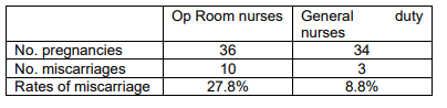
In Example 5.2, data on miscarriage rates for operating room nurses and general duty nurses are compared, with the hypothesis that the miscarriage rate for operating room nurses is higher than that for general duty nurses (

$H_{0} : π_{1} = π_{2}$ versus

$H_{a} : π_{1} > π_{2}$ ).

Op Room Nurses:

Number of pregnancies: 36
Number of miscarriages: 10
Miscarriage rate: 27.8%

General Duty Nurses:

Number of pregnancies: 34
Number of miscarriages: 3
Miscarriage rate: 8.8%

The test statistic

$B$ is calculated as:

$B = \frac{0.278 - 0.088}{\sqrt{\frac{0.1857 \times 0.08143}{36} + \frac{0.1857 \times 0.08143}{34}}}$

Which simplifies to

$B = 2.043$ .

Given the large sample sizes (36 and 34 pregnancies in the two groups), the normal approximation is applied. With a critical value of 1.645 for a one-sided test at the 5% significance level (considering the alternative hypothesis of a “greater than” relationship), the null hypothesis is rejected. The tail area is found to be 0.0205.

This example illustrates the comparison of proportions between two groups and the determination of whether there is a significant difference in the proportions of success.

Due to the simplicity of the test, requiring only the difference in the two proportions, the average of the proportions, and the sample sizes, it’s feasible to create graphs known as nomograms to facilitate testing. These nomograms provide the size of the difference that would be significant at the 5% level, given the sample size and the average proportion. They are frequently utilized in reports of market research surveys like the AMPS and are sometimes presented as ‘margin of error tables.’ These tables list the average sample size and the lower of the two proportions as rows and columns, with the margin of error indicated in the table’s body. Users can look up the approximate average sample size and the lower of the two proportions and read off the size of difference needed to achieve significance.

The confidence interval is calculated as:

$\sqrt{2}$

Where:

and are the standard errors of the proportions.
$z_{1 - α /2}$ is the critical value for the desired level of confidence.
is the significance level.

An alternative (and equivalent) solution to this problem is discussed in section 5.6.

Sample size determination is conducted similarly to previous methods, assuming equal sample sizes and setting the width of the confidence interval to the desired difference to be detected, then solving for $n$ :

$n = (z_{1 - α /2} + z_{1 - β})^{2} (( p ^ ^{1} - p ^ ^{2} ) ^{2} se ( p ^ ^{1} ) ^{2} + se ( p ^ ^{2} ) ^{2})$

Note that this calculation provides the number required in each group.

Comparing proportions in several categories for a single sample

Suppose we have categories labeled as 1, 2, 3, …, , with a proportion $_{}$ of the cases falling into each category. If the null hypothesis is that there is no difference between the categories, then $H_{0} : π_{0, i} = c 1$ , indicating that if there is no difference between the categories, the proportion in each of the categories should be equal. Therefore, under the null hypothesis, we expect to have a proportion of $c 1$ in each category.

To assess this hypothesis, we compare these expected proportions (denoted by ) to the observed proportions (denoted by ). The test statistic is given by:

$χ^{2} = \sum_{i = 1 c} E ^{i} ( O ^{i} - E ^{i} ) ^{2}$

Which follows a chi-squared ( $χ^{2}$ ) distribution. Here, is the Greek letter “chi” and this distribution is known as the chi-squared distribution. The value of the test statistic is then compared to the critical value of a chi-squared distribution with $c - 1$ degrees of freedom (number of categories minus 1).

This test is applicable not only when we expect equal proportions in different categories but also when we “expect” different proportions in different categories, such as when applying Mendelian (genetic) theory.

Example 5.3

Lets consider, the classic experiment on heredity by Mendel concerned four possible groups of first-generation progeny from a crossing of two types of peas.

Mendel’s classic experiment on heredity involved four possible groups of first-generation progeny from a crossing of two types of peas. The observed frequencies were as follows:

Round and yellow: 315
Round and green: 108
Wrinkled and yellow: 101
Wrinkled and green: 32

The theory implied that the ratio of frequencies in these groups should be 9:3:3:1. Tabulating these as observed and expected frequencies for the four groups gives:

\begin{array}{ccc} Group & O_{i} & E_{i} \\ Round and yellow & 315 & 312.75 \\ Round and green & 108 & 104.25 \\ Wrinkled and yellow & 101 & 104.25 \\ Wrinkled and green & 32 & 34.75 \end{array}

The difference between observed and expected values is calculated for each group.

Here, we expect to have a proportion of $\frac{9}{9 + 3 + 3 + 1}$ or $\frac{9}{16}$ of the observations in the first category, giving an expected value of $(556) (\frac{9}{16})$ or 312.75.

This yields a test statistic value of $x^{2} = 0.470$ with 3 degrees of freedom. The probability of getting a $x^{2}$ value greater than or equal to 0.470 by chance alone, for 3 degrees of freedom, is 0.92, indicating that the theory held in practice.

It is worth noting that the theory fitting so well may raise suspicions. While one does not usually formally test to see if the model fits “too well,” suspicions may arise. In this case, there has been conjecture that Mendel’s gardener knew what results he wanted and may have manipulated the outcomes.

Other examples would include queries about whether there were equal proportions of:

Females, or members of a specific race group, or people with disabilities, registered in different faculties.
Four different age groups watching Big Brother.
Unit trusts in different categories yielding returns above a certain level.
Males and females between the ages of 6 and 17 attending schools in rural areas.

Goodness of Fit

Chi-squared tests serve as goodness of fit tests, commonly employed to examine whether data conform to a specific distribution, such as the normal distribution. In the case of the normal distribution, it is established what proportion of data points should fall within certain intervals based on standard normal theory. For instance, it is anticipated that 2.5% of the data should lie below -1.96, another 2.5% between -1.96 and -1.645, and so forth. Alternatively, these proportions can be derived from tables.

To apply the chi-squared test, the data is standardized, and the counts of cases within specified categories are tallied. Expected values are then determined using numbers from normal theory. The alternative hypothesis posits that the distribution is not normal.

Example 5.4:

A random sample of 20 observations is to be tested to determine if it originates from a N(30, 100) distribution. In this scenario, the null hypothesis asserts that the underlying distributions from which the observations are drawn follow N(30,100), while the alternative hypothesis posits that the observations are sourced from a different distribution. To conduct the test, we explore the expected outcomes for a N(30,100) distribution, presuming that the mean and variance are pre-specified.

The ordered numbers in the sample are as follows: 16.3, 17.5, 23.4, 24.3, 25.2, 26.9, 28.4, 29.5, 30.1, 31.7, 32.9, 33.7, 35.8, 35.9, 36.3, 37.3, 39.7, 41.8, 42.3, 45.8.

To execute the test, the range is partitioned into a predetermined number of regions, let’s say 4. These regions are selected so that an equal number of observations is expected in each region, assuming the data conforms to a N(30, 100) distribution. Utilizing tables (refer to Conover, p190 for details), the expected frequencies for each region are determined:

<23.26
23.26-29.99
30.00-36.74
≥36.75

The actual and expected frequencies are as follows:

\begin{array}{ccc} Region & Actual & Expected \\ < 23.26 & 2 & 5 \\ 23.26 - 29.99 & 6 & 5 \\ 30.00 - 36.74 & 7 & 5 \\ \geq 36.75 & 5 & 5 \end{array}

The value of the test statistic is then computed using the formula:

\frac{(2 - 5)^{2}}{5} + \frac{(6 - 5)^{2}}{5} + \frac{(7 - 5)^{2}}{5} + \frac{(5 - 5)^{2}}{5} = 2.8

Another example of a goodness of fit test is assessing whether numbers exhibit randomness. If the numbers are indeed random, and the interval is divided into a certain number of equally sized categories, one would anticipate an equal distribution of numbers across each category. For instance, the expected number of observations in intervals such as (0, 0.1), (0.1, 0.2), …, (0.9, 1.0) would all be identical, each accounting for 10% of the sample. Given that random numbers typically adhere to a uniform distribution, this enables the examination of whether the observed data aligns with this uniform distribution.

Add Your Heading Text Here

Contingency tables serve as a structured way to organize and analyze data when there are two categorical variables of interest. The rationale behind using contingency tables lies in the need to explore potential relationships or associations between these variables. By arranging the data in rows and columns, contingency tables provide a clear visual representation of how the frequencies or counts of observations are distributed across different categories of the two variables.

The main goal of constructing contingency tables is to investigate whether there is a relationship or association between the two categorical variables. This relationship can be examined by comparing the observed frequencies in each cell of the table to what would be expected if there were no relationship between the variables (i.e., if they were independent).

For example, in a study comparing newspaper readership (classified by age group) and preference for certain newspaper sections (classified by content), a contingency table would show the number of individuals falling into each combination of age group and preferred section. Analyzing this table could reveal whether certain age groups are more likely to prefer specific sections of the newspaper, indicating a potential association between age and reading preferences.

Overall, contingency tables provide a structured framework for conducting chi-squared tests, which are commonly used to assess the significance of associations between categorical variables. They offer a systematic approach to exploring relationships in categorical data and are widely used in various fields such as social sciences, epidemiology, market research, and more.

Contingency tables, featuring a single sample and two classifications, are subject to analysis using chi-squared tests. Here are further examples:

Dung Beetle Subspecies and Hatching Time: Investigating differences in hatching time among various dung beetle subspecies.
Newspaper Readership and Age Group: Examining whether readership of a daily newspaper varies across different age groups.
Share Performance and Takeover Type: Assessing if there’s a difference in share performance based on the type of takeover (cash or share buyout).
Age and Preferred Salary Package: Exploring potential associations between respondents’ ages and their preferred salary packages.
Disease Presence: Studying the potential co-occurrence of two diseases to determine if they are associated or occur independently.

Each example can be depicted in an RxC contingency table format, with rows representing categories for the first classification and columns for the second classification. The table structure is outlined as follows:

	Col 1	Col 2	…	Col C	Total
Row 1	O11	O12	…	O1C	n1
Row 2	O21	O22	…	O2C	n2
…	…	…	…	…	…
Row R	OR1	OR2	…	ORC	nR
Total	n.1	n.2	…	n.C	N

Here, N represents the total number of observations, n.i denotes the total number of observations in the i’th row, and n.j signifies the number of observations in column j. The observations are distributed across the cells of the table based on their classifications.

Contingency tables serve as a structured way to organize and analyze data when there are two categorical variables of interest. In Example 5.5, the scenario involves comparing the opinions on smoking among students from different home regions. The purpose of constructing a contingency table in this context is to examine whether there is an association between students’ home regions and their opinions on smoking.

Under the null hypothesis that there is no difference in opinion among students from different regions, the expected proportion of students holding each opinion category should be similar across all regions. The contingency table shows the observed counts of students in each combination of home region and opinion category, along with the expected counts if there were no association between these variables.

To assess whether there is an association between home region and opinion on smoking, a chi-squared test is performed. The test statistic compares the observed counts to the expected counts in each cell of the contingency table. In Example 5.5, the test statistic yields a value of 80.88, which is compared to the critical value from a chi-squared distribution with degrees of freedom determined by the dimensions of the contingency table. Since the test statistic exceeds the critical value, the null hypothesis of no association between home region and opinion on smoking is rejected, indicating that there is indeed an association between these variables.

The chi-squared contingency table test relies on the approximation of the test statistic’s distribution to a chi-squared distribution. However, this approximation may be poor if some of the expected counts are small. Therefore, it is recommended that all expected counts be greater than 1, and not more than 20% should be less than 5. If these conditions are not met, combining categories may be necessary.

Overall, contingency tables provide a systematic framework for assessing associations between categorical variables, and the chi-squared contingency table test is a valuable tool for determining the significance of these associations.

Fisher’s Exact Test

Fisher’s Exact Test is a valuable method of analysis, especially when dealing with small samples or a 2×2 contingency table where both row and column totals are pre-specified. In situations like these, where the sample size is small or the data structure is specific, Fisher’s Exact Test provides an exact approach to test for associations between categorical variables.

An iconic example of Fisher’s Exact Test is illustrated in a statistical experiment conducted by R.A. Fisher, where the objective was to determine whether a colleague could distinguish between cups of tea where milk was added first versus cups where tea was added to milk. In this experiment, eight cups of tea were prepared, with four having milk added first and four having tea added to milk. Fisher’s Exact Test allows for the evaluation of whether there is a significant association between the order of adding milk and the ability to correctly classify the cups.

Unlike chi-squared tests, Fisher’s Exact Test does not rely on large sample approximations, making it suitable for small sample sizes. However, one challenge with small samples is the difficulty of detecting significant associations, particularly when there are only a few observations.

Fisher’s Exact Test can also be applied to 2×2 contingency tables where only one of the row or column totals is fixed, or when neither are fixed. In such cases, the test is “conditional on” the observed values of the non-fixed totals, treating the table as if the row and column totals were pre-specified. While other exact tests exist for 2×2 tables with non-fixed totals, they are not as widely available as Fisher’s Exact Test.

Additionally, there are several correlation coefficients suitable for contingency tables, providing further insights into the relationships between categorical variables. These coefficients offer measures of association or dependence tailored to the specific structure of contingency tables, enhancing the understanding of the relationships between the variables under study.

Contingency tables: 2 or more samples, 1 variable

Contingency tables provide a structured framework for analyzing categorical data, especially when investigating associations between two categorical variables. In scenarios where the row totals are fixed, such as studying the effectiveness of vitamin C in preventing colds, or comparing the preferences of skiers who received a placebo versus those who received ascorbic acid, contingency tables offer a methodical approach to categorizing observations and evaluating relationships between variables.

For instance, in the study evaluating the effectiveness of vitamin C in preventing colds, skiers were categorized based on whether they received a placebo or ascorbic acid, and whether they developed a cold or not. This categorization forms the basis of the contingency table, with fixed row totals representing the total number of observations for each treatment group.

Similar investigations, such as examining subspecies of bees based on hive size, comparing respondents’ reactions to different versions of a question, or assessing preferences for flexi-time among employees from multiple firms, can all be analyzed using contingency tables. These tables organize the data into rows and columns, with fixed row totals representing the total number of observations within each category.

In Example 5.2, concerning miscarriage rates for different categories of nurses, the data can be structured into a contingency table to test for an association between miscarriage rates and the area of work. Whether analyzing proportions directly or testing for associations between variables, the contingency table framework facilitates systematic analysis and hypothesis testing.

To conduct hypothesis tests using contingency tables, the chi-squared test statistic is commonly employed. By comparing the observed frequencies to the expected frequencies under the null hypothesis, researchers can assess whether there is evidence of an association between the variables of interest. In Example 5.2, the test statistic is calculated to evaluate whether there is an association between miscarriage rates and the place of work, leading to a conclusion regarding the differences in miscarriage rates between the two workplaces.

Contingency tables are widely used in various fields, including market research and epidemiology, where categorical data are prevalent. Their structured format allows researchers to organize and analyze data effectively, leading to insights into the relationships between categorical variables.

The following examples illustrate the versatility of contingency tables in analyzing categorical data across various contexts:

Ownership of a refrigerator by demographic factors: Cross-tabulating ownership of a refrigerator with variables like education level, living standard measure (LSM), or access to electricity allows researchers to examine patterns of appliance ownership across different socioeconomic groups.
Agreement or disagreement with statements: Comparing responses to statements like “families should do things together” or “shoplifting food is unethical even if you are hungry” against demographic factors such as age, income, or gender enables researchers to explore attitudes and beliefs within different population segments.
Reading habits and consumer behavior: Analyzing whether individuals read a weekly magazine in the last week based on household characteristics like the number of cars or usage of financial products like savings accounts provides insights into consumer behavior and media consumption patterns.
Share price performance: Investigating whether the price of a share increases two weeks after being issued allows researchers to assess the short-term performance of newly issued shares, potentially identifying trends or anomalies in the market.
Hospitalization and health outcomes: Examining the number of weeks spent in the hospital among children categorized by HIV status provides valuable information on the relationship between health conditions and healthcare utilization.
Ecological studies: Studying the number of dung beetles from different species found in dung-pats from various types of animals helps ecologists understand dung beetle behavior and ecological interactions within different ecosystems.

In each of these examples, contingency tables serve as a powerful tool for organizing and analyzing categorical data, allowing researchers to identify patterns, associations, and trends across different groups or categories. By systematically organizing data into rows and columns, researchers can conduct hypothesis tests, identify significant relationships, and draw meaningful insights to inform decision-making and research outcomes.

Summary of tests for categorical data

This chapter delves into statistical methods tailored for analyzing categorical data. We began with tests for a single proportion, useful for comparing sample proportions against known values or population proportions. Then, we explored chi-squared tests, which encompass goodness of fit tests to assess observed frequencies against expected distributions and tests for independence to evaluate associations between two categorical variables in contingency tables.

Contingency tables were highlighted as a crucial tool for organizing categorical data into rows and columns, facilitating the examination of relationships between variables. Fisher’s exact test was introduced as a valuable option for small sample sizes or fixed row and column totals in contingency tables.

Throughout the chapter, numerous applications of these methods were discussed, spanning market research, epidemiology, and social sciences. Examples included demographic cross-tabulations, agreement/disagreement assessments, and product preference analyses.

By grasping these statistical techniques and their interpretations, researchers can derive meaningful insights into categorical data relationships, enabling informed decision-making across diverse domains.