In many cases, the primary aim of a study is to determine if there are differences between two or more groups. Therefore, when examining data, researchers typically have a hypothesis they want to validate or reject based on the collected data.
Examples include:
- Investigating whether there is a difference in test scores between students who received tutoring and those who did not.
- Examining whether there is a variation in productivity levels among different departments within a company.
- Testing if there is a disparity in customer satisfaction ratings between two different service providers.
- Analyzing whether there are differences in recovery times between patients who received different treatments.
- Assessing if there is a variation in energy consumption between households using different heating systems.
In some cases the study is exploratory with no definite hypothesis: In these kind of studies, researchers aim to gain insights and generate hypotheses rather than test specific hypotheses. These studies are often conducted when little is known about a particular phenomenon or when existing theories are insufficient. Researchers may collect data without predetermined hypotheses to explore patterns, relationships, or trends within the data. examples include:
- Conducting interviews or surveys to explore people’s attitudes, behaviors, or experiences in social science research.
- Analyzing experimental data to identify unexpected correlations or patterns in scientific research.
- Exploring patterns or trends within large datasets without predetermined hypotheses.
- Studying uncharted areas or phenomena to generate new ideas and hypotheses.
- Observing natural phenomena or events to understand underlying patterns or relationships.
Population versus sample
The term “population” refers to all relevant items in a study. Typically, the goal of the study is to make a statement about this entire group. For instance, we might want to assert that female university students achieve higher grades than their male counterparts. However, examining every single element in the population is often impractical, especially if the population is extensive (imagine trying to collect the grades of every university student globally). Instead, researchers use a sample—a subset of the population. This sample is then analyzed to test the hypothesis of interest.
Let’s say we’re conducting a study to investigate whether there’s a significant difference in the grades obtained by male and female university students. Instead of trying to collect grade data from every university student globally, which would be impractical, we select a representative sample of students. This sample would ideally include both male and female students from various universities and academic disciplines. By analyzing the grades of this sample, we can draw conclusions about the larger population of university students regarding gender-based differences in academic performance.
Other examples include:
- If you conduct a survey on job satisfaction among employees in a specific company in Johannesburg, your findings will only represent the opinions of those employees and may not apply to workers in other companies or regions of the country.
- When analyzing crime rates in a particular province, such as Gauteng, the data will reflect only the incidents reported within that province and may not accurately represent crime rates in other provinces like KwaZulu-Natal or Western Cape.
- If you study the impact of a government policy on education outcomes in a rural area of the Eastern Cape, your findings will pertain only to students and schools in that specific region and may not be applicable to urban areas or other provinces.
When testing hypotheses about population means or proportions, it’s crucial to consider the variability within the data. This means that simply comparing the means of two groups isn’t sufficient; you also need to account for the spread of the data. Since the actual parameters of the populations are typically unknown, we rely on estimates from the sample data. The sample mean and variance are used to estimate the corresponding parameters of the population.
Consider these examples:
Educational Intervention Study: When comparing the mean test scores of students under different teaching methods, simply comparing the averages may not be sufficient. For instance, if the mean test score of students in the new teaching method group is higher than that of the traditional method group, it might suggest that the new method is more effective. However, if the variability (spread) of scores within each group is large, it could indicate that some students performed exceptionally well while others struggled, regardless of the teaching method. In this case, the effectiveness of the new method may not be as clear-cut as suggested by the mean scores alone.
Product Testing: In comparing satisfaction ratings of two smartphone brands, if the mean satisfaction rating of one brand’s users is higher than the other, it might indicate that users generally prefer that brand. However, if there is a large variability in satisfaction ratings within each brand’s user group, it suggests that individual preferences vary widely. This variability could influence marketing strategies or product improvements to cater to different user preferences.
Medical Trials: When comparing the effectiveness of two drugs in a clinical trial, a higher mean improvement in symptoms for one drug compared to the other might suggest that it’s more effective. However, if there’s considerable variability in symptom improvement within each drug group, it indicates that individual responses to the drugs vary. This variability could influence decisions about treatment options and patient care.
Normal Distribution
Think about how observations usually aren’t perfectly precise. What we actually see is the real measurement, but there’s also some random variation mixed in. Many statistical tests assume that the random fluctuations around an observation can make it either higher or lower than the true value with equal likelihood. This creates a symmetrical pattern where observations are spread out evenly on both sides of the true value.
let’s consider the example of measuring the height of a group of students. If we assume that random errors in measurement can make a student’s height appear either slightly taller or slightly shorter than their actual height, then on average, these errors should balance out. This means that some students might appear taller than they are due to measurement error, while others might appear shorter, but overall, the errors should roughly cancel each other out, resulting in a symmetric distribution of measured heights around the true average height of the students.

In the histogram shown in figure 2.1, it represents the heights of approximately 1000 first-year male students at Wits University. The majority, roughly 95%, fall within the range of 1.6 meters to 2.1 meters. As anticipated, the observed heights display a relatively symmetrical distribution around the mean height. Most heights cluster around the mean, with few extremely small or large heights. If we were to create a smoothed version of this histogram, it would resemble figure 2.2.
The normal or Gaussian distribution is the most frequently observed distribution with the characteristic of symmetry. One key reason for its widespread use is that it’s often found that the means of samples follow a normal distribution pattern, as explained in section 2.3.
In the normal distribution, knowing the mean and variance is enough to effectively summarize the data from that distribution.
Normal distributions with varying means and variances can be expressed mathematically using a distribution with a mean of zero and a standard deviation of one. This allows for the use of a single set of tables to look up results for any normal distribution by converting it into a standardized normal distribution, instead of needing separate tables for each possible combination of mean and variance. For example, suppose we have two normal distributions: one with a mean of 10 and a standard deviation of 2, and another with a mean of 20 and a standard deviation of 4. We can convert these distributions into standardized normal distributions by subtracting the mean from each value and then dividing by the standard deviation. This process allows us to compare data from both distributions using a single set of standardized normal distribution tables.
Distribution of the mean of a set of data
A significant rationale behind focusing on the normal distribution is that, when dealing with large samples, the AVERAGE of a dataset from most distributions tends to follow a normal distribution. This phenomenon, demonstrated by the central limit theorem, applies to large sample sizes across various scenarios, even if the original data distribution is not normal. Typically, in practice, “large” refers to sample sizes exceeding 40, although some sources indicate that 30 is considered sufficient.
As previously mentioned, the hypothesis we often seek to test concerns the mean. For instance, in the case of the heights of first-year male students at Wits, we might want to determine if the average height is 1.7m. To conduct such a test using our sample, we must assess the mean in relation to the variability surrounding it. We recognize that if we had taken a slightly different sample, we would have obtained a slightly different mean. Therefore, we need to establish the distribution for the mean of samples from the population of first-year male students and compare it to 1.7m. However, in practice, we typically have only one sample. Conceptually, we can construct this distribution by drawing numerous samples, calculating the mean of each sample, and then creating a histogram of these means. Although we do not perform this procedure in practice, understanding these concepts is crucial as they underpin the principles of statistical analysis.
We can conceptually create this distribution by taking numerous samples, calculating the mean of each sample, and then plotting a histogram of these means. However, in practice, we don’t carry out this process. Instead, we rely on established distribution properties. Nonetheless, exploring what occurs in this thought experiment is valuable as it helps elucidate important concepts.
Drawing samples of 10 students at a time and calculating the mean for each sample would likely result in a wide range of mean values, although the average of these means would still be close to the true mean. Conversely, if we took samples of 100 students at a time, we would anticipate much less variation in the calculated means.
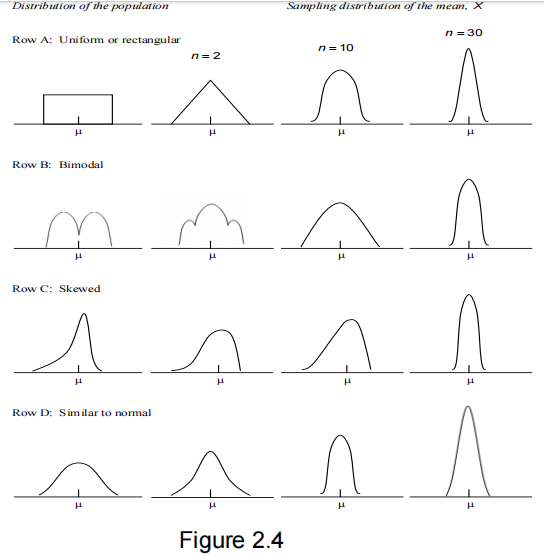
In figure 2.4 from Dawson-Saunders and Trapp (1990), row C demonstrates an experiment. The first plot exhibits a skewed distribution, where most data points cluster around a central value, but there’s a slight chance of obtaining very low figures. The second plot illustrates the process of repeatedly drawing samples of 2 observations from this distribution, calculating the mean for each sample, and plotting these means to derive the distribution of means. While still skewed, this resulting plot shows less skewness than the initial distribution. The third figure displays the distribution of means for samples of size 10 (sampling 10 observations at a time), while the last figure depicts the distribution of means for samples of size 30. As sample size increases, the distributions become more symmetrical, resembling the normal distribution in figure 2.3.
This process was repeated for three additional distributions:
- Row A: the uniform or rectangular distribution, where all data falls between two numbers, with each data point having an equal chance of occurring anywhere within this range.
- Row B: a bimodal distribution, indicating data arising from two separate but overlapping distributions.
- Row D: the normal distribution.
These plots demonstrate examples of how the means of large samples tend to be normally distributed, sharing the same mean as the initial distribution.
Now focusing on Row D, the normal distribution: the initial distribution of observations (first plot) is normal, as are the subsequent three plots. However, the variability among the means of samples of size 2, 10, and 30 will be much lower than that in the original dataset due to the averaging process.
In statistical terms, we typically refer to the standard error rather than the standard deviation of an estimator like a mean. The term “standard deviation” is typically used for data itself.
The sample mean also possesses the characteristic of being an unbiased estimate of the population mean. This indicates that as we draw larger samples, not only do the estimates of the sample means become more consistent, but they also approach closer and closer to the mean of the population from which the data are collected.
Confidence IntervaIs
While summarizing a dataset with the mean value is common, it often results in loss of information. A more sensible approach is to provide a range of values within which we expect the true mean to fall, known as a confidence interval.
Let’s say we want to estimate the mean weekly weight gain of piglets on a certain diet. We have data on weight gain from 16 piglets over a one-week period. Our goal is to make a statement about the range of weight gains expected from healthy piglets fed this specific diet.
For instance, consider the following weight gains (in grams) on the supplemented diet: 448, 229, 316, 105, 516, 496, 130, 242, 470, 195, 389, 97, 458, 347, 340, 212.
For now, let’s assume we already know the standard deviation of the weekly weight gains of piglets based on previous studies concerning diets. We’ll assume it to be 120 grams. The mean weight gain of the 16 piglets in this study is 311.9 grams. However, we understand that if we were to repeat the study, we would likely obtain a different mean weight gain.
However, we can estimate the range within which the mean weight gain is likely to fall by using a formula for the distribution of the sample mean:

When we standardize the sample means, we obtain:

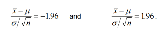
With the knowledge that 95% of the observations from a normal distribution lie between -1.96 and 1.96 standard deviations from the mean, we can compute a 95% confidence interval for the mean weight gain.
It’s worth noting that while we’ll stick with a 95% confidence level for consistency, it’s common to see confidence levels set at 90% or 99% in various contexts. These are among the standard choices for confidence levels.
Given that 95% of values from a standardized normal distribution fall between -1.96 and 1.96, we can anticipate that 95% of z-values will lie within this range as well. To establish a confidence interval for the population mean μ, expressed in terms of the sample mean x, the population standard deviation σ, and the sample size n (all presumed known for now), we set z to -1.96 and solve for μ, then set z to 1.96 and solve for μ again. This entails solving the equations:
With a sample size of n=16, a mean of 311.9, and an assumed σ=120, this interval extends from:
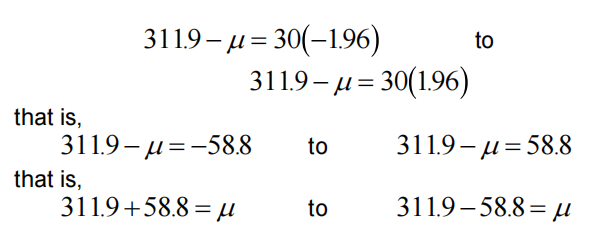
providing a 95% confidence interval for μ of 253.1 to 370.7, typically denoted as (253.1, 370.7).
This implies that, while we can’t determine precisely how close the mean obtained from this sample, 311.9, is to the true mean, we can be 95% confident that it falls within two standard deviations of the true mean. Thus, in 95% of samples drawn, we anticipate the unknown population mean μ to fall within this confidence interval It’s important to note that the 95% confidence interval derived from the data is symmetric around the estimated mean. Consequently, the estimated mean will consistently fall within the confidence interval.
Hypothesis Testing
Confidence intervals can also serve as a tool for hypothesis testing. If the objective of the study was to determine whether the mean weight gain on a particular diet differs from a predetermined value, such as 200 grams, we can frame this as a formal hypothesis: we aim to ascertain if the population mean, from which the sample was drawn, significantly deviates from a specified value (in this case, if the mean weekly weight gain on the diet equals 200 grams or not, i.e., if μ=200 or not). Given that 200 lies outside the calculated confidence interval, we can reasonably infer that the true mean is unlikely to be 200.
More formally, hypothesis testing involves establishing a NULL HYPOTHESIS and an ALTERNATIVE HYPOTHESIS. The null hypothesis (denoted by H0) suggests no difference exists. Thus, we seek to assess the null hypothesis that the population mean, from which the sample was drawn, aligns with a mean of 200 grams, represented as H0: µ = 200. Conversely, the alternative hypothesis posits that the population mean is not in line with a mean of 200 grams, denoted as Ha: µ ≠ 200 grams.
The alternative hypothesis will be consistently referred to as Ha in this text. While other texts may use the terminology H1, the focus here remains on the alternative hypothesis, as it typically represents what one aims to demonstrate. Therefore, the primary interest lies in establishing that:
- Employees who work remotely exhibit higher job satisfaction levels than those who work in the office.
- Using environmentally friendly packaging results in a higher percentage of consumers choosing a product over competitors with conventional packaging.
- Students who participate in extracurricular activities achieve higher grades than those who do not engage in any extracurriculars.
- Increased investment in employee wellness programs leads to a reduction in absenteeism rates compared to companies without such programs.
- Companies that offer flexible work hours experience higher employee retention rates than those with rigid work schedules.
- Implementing a recycling program in schools leads to a decrease in overall waste production compared to schools without recycling initiatives.
- A new social media marketing campaign results in a higher number of website visits and conversions compared to previous campaigns.
- Regular exercise leads to more significant improvements in mental health outcomes compared to medication alone.
- Adopting agile project management methodologies results in faster project completion times compared to traditional waterfall approaches.
- Providing incentives for carpooling leads to a reduction in traffic congestion and air pollution compared to individual commuting.
It’s challenging, and in fact impossible, to develop statistical tests to evaluate these ambiguous hypotheses because the term “higher than” lacks precise definition. Its interpretation varies from person to person. While one might suggest “any difference,” it’s improbable that someone would invest in additional statistical training if it only marginally increases their average mark by 0.5%. However, for a substantial improvement of 10% or 20%, pursuing such training might be worthwhile.
Tests for precise hypotheses, like whether people have an equal preference for Coke or Pepsi, are straightforward to establish. In this scenario, the null hypothesis (sometimes termed the ‘dull hypothesis’) posits that the average rating for Coke and Pepsi in the population is 5 on a scale of 0-10. Therefore, if data collection reveals evidence contradicting the equal preference assumption (e.g., an average rating of 7.5), we reject the null hypothesis and accept the alternative hypothesis that people do not share an equal preference for Coke and Pepsi.
These examples focus on comparing two or more groups, a topic we’ll delve into shortly. For now, to clarify some of the underlying concepts of hypothesis testing, we’ll continue with the scenario of testing a single sample to determine if the mean equals a predefined value. Additionally, we’ll maintain the assumption that the standard deviation is known for the time being.
As mentioned earlier, one method of testing whether the population mean (µ) equals 200 is to determine if 200 falls within the 95% confidence interval. Since it doesn’t, if the null hypothesis (H0: µ = 200) is true, we must have encountered the rare circumstance of drawing one of the 5% of samples where the true population mean lies outside the 95% confidence interval obtained from the data. Given the low probability of this occurrence, we explore alternative explanations. The most apparent one is that the null hypothesis is incorrect. Therefore, we conclude that the null hypothesis H0: µ = 200 is inaccurate and accept the alternative hypothesis Ha: µ ≠ 200. It’s important to acknowledge that there’s a 5% chance of error in this conclusion. Hence, we state that we reject the null hypothesis at the 5% significance level.
NB: It’s essential to differentiate between confidence intervals and hypothesis testing. In confidence intervals, like a 95% confidence interval, we express our confidence that the true population mean lies within a specific range. However, in hypothesis testing, such as a test at the 5% level, we focus on the risk of error when rejecting the null hypothesis. This 5% level represents the area beyond the interval where we anticipate the true mean to lie.
Another method for testing the hypothesis involves revisiting the formula for the distribution of the mean:

and instead of solving it to derive a confidence interval, we utilize this directly to provide a test for the hypothesis.
Example 2.2 (continued) For the piglets on the supplemented diet, we have determined the mean weekly weight gain in our sample to be 311.9, with 16 observations. Additionally, we’ve assumed the population standard deviation, σ, to be 120, and our hypothesis to test is μ=200. Therefore,

Now that we’ve calculated a value above 1.96, we know that only 5% of samples drawn from a standard normal distribution would yield a value this large by chance alone, if the null hypothesis is true. Therefore, we reject the null hypothesis and accept the alternative hypothesis at the 5% significance level, indicating that we are taking a 5% chance of being wrong in drawing this conclusion.
Using this procedure implies that we can expect to draw the wrong conclusion in 5% of cases. Therefore, it’s crucial to consider how large a risk you’re willing to take when drawing your conclusion, as this varies from one situation to another.
For instance, initial screening tests for diseases like HIV might be conducted with a relatively lenient threshold, perhaps around 10% or higher, to ensure the detection of all potential cases. However, the follow-up tests, which are usually more precise but also more expensive, may employ a much stricter threshold, perhaps as low as 0.1%. While a 5% significance level is commonly used for testing in this text, it’s important to carefully consider the actual testing level in any real-world scenario.

We term this the TEST STATISTIC: As mentioned earlier, we check whether the test statistic exceeds 1.96 or falls below -1.96. If it does, we conclude that we reject the null hypothesis in favor of the alternative hypothesis at the 5% significance level. This threshold value (in this case, 1.96, derived from the normal distribution) is also referred to as the critical value.
In simpler terms, we can say: reject the null hypothesis if the absolute value of z is greater than 1.96, where the absolute value of z means ignoring the sign of the calculated value of z (for example, |2| = 2, and |-3| = 3).
In summary, this complex procedure involves several steps:
- We start with our sample data, which represents a subset of the overall population.
- We set up a null hypothesis (H0: µ = 200) and an alternative hypothesis (HA: µ ≠ 200).
- We choose a significance level for testing, typically 5%.
- Assuming we know the population standard deviation (σ = 120), although this assumption will be revisited later.
- We make the assumption that the data are approximately normally distributed.
- We calculate a test statistic using our sample data.
- We compare this test statistic to the critical value of 1.96, determined from the knowledge that the test statistic follows a standard normal distribution.
- If the calculated test statistic exceeds the critical value, we note that this occurrence is expected only 5% of the time under the assumption of a population mean of 200 and a standard deviation of 120.
- Consequently, we conclude that it is unlikely and opt for the alternative possibility, suggesting that the population mean differs from 200.
We can illustrate this graphically as follows:

We understand that in a standard normal distribution (N(0,1)), 95% of values fall between -1.96 and 1.96, with 2.5% below -1.96 and 2.5% above 1.96. Given that our test statistic is greater than 1.96, it falls within a zone where we anticipate obtaining values only 5% of the time. This specific area is termed the CRITICAL REGION.
With modern computing capabilities, we can employ more advanced methods. Rather than simply checking if the test statistic falls within the critical region, we can calculate the actual probability of obtaining a test statistic of 3.73 or greater, assuming the null hypothesis is true. In essence, we determine the probability associated with a critical value of 3.73.
The probability of obtaining a value of ∣z∣ equal to or greater than 3.73 (the p-value or tail area) is calculated to be 0.0001916 (using a computer). This implies that we anticipate observing a test statistic as extreme as 3.73, purely by chance, in only 0.01916% (or 0.0001916 multiplied by 100) of instances when the null hypothesis is true. Consequently, we can reject the null hypothesis not only at the 5% significance level but also at the 1% and even the 0.05% significance levels in this example.
Another interpretation of the p-value is that it represents the probability level at which the decision regarding �0H0 will be on the borderline between acceptance and rejection. In this context, if we aim to test at any level higher than 0.01916% (meaning we’re willing to accept at most a 0.01916% risk of making an error in rejecting the null hypothesis), then we would reject the null hypothesis in this example. However, if we’re not comfortable with this level of risk and prefer a smaller chance, such as 0.01%, then we would refrain from rejecting the null hypothesis. The same principle applies if we aim for an even lower chance, such as 1 in 10,000, or 0.01%.
Another example: Let’s say our calculated p-value or tail area is 0.072. Because this value is greater than 0.05, we cannot reject the null hypothesis at the 5% significance level. However, it is less than 10%, so we can reject the null hypothesis at the 10% level of significance. This method of hypothesis testing, where we consider the p-value rather than solely relying on confidence intervals, is commonly employed in research literature.
There are several reasons for this approach:
- Conducting tests at different significance levels, like 5%, 1%, and 0.1%, isn’t necessary. The test outcome remains consistent unless the acceptable risk changes.
- When dealing with various distributions, critical values may vary and become complex. However, relying on p-values ensures consistent interpretation across different distributions.
- Using confidence intervals for testing isn’t always suitable, especially in more complex scenarios like one-sided tests. Therefore, relying on p-values offers a more versatile approach to hypothesis testing.
Therefore, the null hypothesis will always be rejected if the p-value provided by the statistical package is smaller than the chosen significance level. Conversely, if the p-value exceeds the specified significance level, we will not reject the null hypothesis. For instance, if we are testing at the 1% level and obtain a p-value of 0.03741, we would retain the null hypothesis.
One sided versus two sided tests
In Example 2.2, the alternative hypothesis was formulated as “not equal to,” indicating the possibility of either higher or lower values. This type of hypothesis test is termed a TWO-SIDED TEST. Alternatively, if our interest was solely in determining whether the diet leads to greater weight gain, we could have employed a ONE-SIDED TEST, where the alternative hypothesis would be formulated as Ha: µ > 200 grams, focusing exclusively on higher values.
In a one-sided test, the cutoff value is different from that used in Example 2.2. For a one-sided test, where the alternative hypothesis focuses solely on values greater than a certain threshold (such as µ > 200 grams), we are only concerned with the critical value above which 5% of the distribution lies. In contrast, in a two-sided test, we seek two values that encompass 5% of the distribution each, one above and one below the center. Since the normal distribution is symmetrical, for a one-sided test, we look for the value z above which 2.5% of the distribution lies. This value is approximately 1.645.
For the piglets on a supplemented diet example, we aim to assess whether the weight gain is significantly greater than 200 grams, thus the null hypothesis states that the weight gain equals 200 grams, while the alternative hypothesis posits that it exceeds 200 grams. The test statistic remains the same.
With x=311.9, n=16, and still assuming σ=120, the test statistic remains at 3.73. However, the probability of obtaining a z value greater than 3.73 is now 0.0000958. Thus, the computer output will indicate that the one-sided test for Ha:μ>200 has a probability of 0.0000958. This contrasts with the two-sided test probability of 0.0001916, which is the sum of the probabilities of getting a value greater than 3.73 and less than -3.73. Therefore, for a one-sided test, we would reject the null hypothesis at the 0.0000958 or 0.00958% significance level, instead of the 0.01916% level obtained for the two-sided test. It’s important to note that the alternative hypothesis must be determined before examining the data; otherwise, the probability statements lose validity.
To illustrate the distinction between one and two-sided tests, let’s refer to Figure 2.6, which displays a standard normal distribution N(0,1). In the context of a one-sided test, as depicted on the right-hand side of the figure, we’re interested in examining whether the mean is higher than a pre-specified value. If we’re conducting the test at the 5% level (using a significance level of 0.05), we need to identify the critical value above which 5% of the distribution lies. For a normal distribution, this critical value is typically denoted as z1−α, indicating the cutoff beyond which a proportion α of the distribution resides. Specifically, for =0.05 and a one-sided test, 0.95=1.645 serves as the critical value, signifying the threshold above which 5% of the normal distribution falls.
In a two-sided test, the critical values are -1.96 and 1.96, as illustrated in the left-hand side of the figure. The region under the curve beyond 1.96 comprises 2.5%, symmetrically mirrored by the 2.5% below -1.96. Therefore, one would use z0.025=−1.96 to denote the critical value below which 2.5% of the normal distribution lies, and z0.975=1.96 to indicate the critical value above which 2.5% of the normal distribution exists. This indicates that there’s a 5% chance of obtaining a value greater than 1.96 or less than -1.96 purely by chance, given that the sample originates from the pre-specified standard normal distribution.
It’s important to note that when tests are conducted using a computer, and the alternative hypothesis is specified as “not equal to,” “less than,” or “greater than,” the computer output will automatically provide the correct p-value for the situation. In such cases, there’s no need to manually divide or multiply by 2. However, some software packages might only offer a “not equal to” option for certain tests. In such instances, obtaining the one-sided value may involve dividing the provided value by 2. This is why the methodology is described in such detail here, to ensure clarity and accuracy in interpretation. see below:

One sample T test
In most real-life scenarios, assuming that the variance is known beforehand is highly unrealistic. Typically, it’s estimated from the available data. In the calculation mentioned above, the population standard deviation σ is replaced by the sample standard deviation s, resulting in a modified test statistic:

This alteration implies that the normal distribution is no longer applicable, and instead, the t-distribution must be employed. The t-distribution shares similarities with the normal distribution in being symmetrical but possesses thicker tails, especially for smaller sample sizes. As the sample size n increases, the t-distribution approaches the normal distribution asymptotically. Beyond a sample size of 1000, the two distributions become practically indistinguishable, and even for sample sizes exceeding 40 (or sometimes 30), the disparities are minimal. Consequently, t-tables frequently cease at around 30 or 40.
The challenge with utilizing the t-distribution is that the critical values, which indicate the thresholds above or below which certain proportions of the data lie, vary according to the sample size. To determine these values from tables or computational tools, it’s necessary to calculate the degrees of freedom. For the one-sample t-test, this entails subtracting 1 from the number of observations. The rationale behind this is that when computing the test statistic, we estimate the mean and employ it in the variance calculation. Given the knowledge of n−1 observations and the mean, we can deduce the remaining observation. Consequently, we are left with n−1 independent pieces of information for estimating the variance.
Example continued: The sample size being 16, the degrees of freedom amount to 15. To identify the critical value of the t-distribution above which 5% of the observations reside (indicating that 95% lie below it), we consult a table of critical values. Below is a section of such a table, listing the degrees of freedom in the first column, and the corresponding critical values for α=0.05 and α=0.025:

For 15 degrees of freedom and a one-sided test, the critical value t0.95,15 is 1.753.
For a two-sided test, we need to find the value t such that 2.5% lies above it, and 2.5% lies below −t. To obtain the critical value for which 2.5% lies above it, 97.5% will lie above that point. Thus, we look up t0.975,15, which equals 2.131. Since the t-distribution is symmetrical, the critical value for which 2.5% lies below it is −2.131.
To calculate the 95% two-sided confidence interval, we use the sample mean xˉ=311.9 grams, the sample standard deviation s=142.8 grams, and the critical values t0.025,15=2.131 and t0.975,15=−2.131 for a two-sided test with 15 degrees of freedom.
The formula for the confidence interval is:

Now, let’s calculate the confidence interval.


So, the 95% two-sided confidence interval is approximately (235.8233,387.6767)(235.8233,387.6767) grams. Computing the test statistic, we obtain

Since this value is greater than the critical value of 2.131, we reject the null hypothesis that the population mean is 200 grams, at the 5% level.

Using the Statistical analysis software (SAS) to obtain the actual p-value, we find it to be approximately 0.0068. Therefore, we can reject the null hypothesis H0:μ=200 in favor of the alternative hypothesis at the 0.68% level, or equivalently, at the 10%, 5%, and 1% levels.
The p-value obtained now is higher compared to the previous calculation where we assumed the population standard deviation to be 120 grams. There are two main reasons for this difference. First, we used the sample standard deviation of 142.8 grams instead of the assumed population standard deviation of 120 grams, which led to a smaller test statistic. Second, we used a higher critical value of 2.131 from the t-distribution instead of 1.96 from the normal distribution, indicating more uncertainty due to estimating the variance from the sample.
If we were conducting a one-sided test, evaluating the null hypothesis H0: μ = 200 against the alternative hypothesis HA: μ > 200, the tail area would be 0.0034. Therefore, in a one-sided test, we could reject the null hypothesis at the 0.34% significance level.
Two Sample T test
Let’s say we did an experiment with two groups of piglets. One group got a regular diet, and the other got a diet with extra supplements. Here’s the data we got:
Supplemented diet group:
- Piglet weight gains: 448, 229, 316, 105, 516, 496, 130, 242, 470, 195, 389, 97, 458, 347, 340, 212
Standard diet group:
- Piglet weight gains: 232, 200, 184, 180, 265, 125, 193, 322, 211.
We want to see if there’s a difference in weight gain between the two groups. We compare the average weight gain of the two groups to figure this out.
The average weight gain on the supplemented diet is 311.875, while the average weight gain of the control group is 212.444. Our main idea is to test if there’s no difference in weekly weight gain between the two diets in the populations, suggesting that any differences are just due to natural variations among piglets and not because of the diets. Let’s assume our alternative hypothesis is that the weekly weight gain is higher on the supplemented diet. So, our alternative hypothesis is HA:u1 > u2.
Now, to proceed with our test, we need an estimate of the standard deviation. We have two estimates available: one from group 1 (142.8) and one from group 2 (56.114). Initially, let’s assume that both groups of piglets come from the same population, so both 142.8 and 56.114 are estimates of the population standard deviation of the groups. The most straightforward estimate of the variance in this case is the pooled estimate of variance, also known as the mean square error or MSE
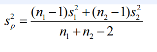
For the given data, this calculation yields sp=119.98, where s1=142.8, s2=56.114, n1=16, and n2=9. The test then is:
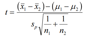
If we assume that the null hypothesis H0:μ1=μ2 holds (which is typical), the formula simplifies to:


where μ1 is the population mean for the supplemented diet, and μ2 is the population mean for the standard diet. This gives:
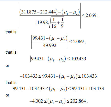
Note that this interval includes zero, and remember that confidence intervals are typically two-sided. If we recall, the hypothesis test would not have been rejected at the 5% level in the case where we were considering a two-sided alternative.
If we had wanted a one-sided confidence interval, we would have used the critical value 1.711. For a “less than” alternative, the confidence interval would have ranged from minus infinity to 184.97, as we’re only interested in obtaining a value above which we’re 95% certain that the true mean will lie. For a “greater than” alternative, the confidence interval would go from 13.89 to infinity. Since this range is greater than zero, we would reject the null hypothesis that the two means are equal, favoring the alternative hypothesis that the mean on the supplemented diet is higher than that on the standard diet.

In any analysis, it’s crucial to verify if the assumptions made are reasonable. In this case, one assumption was that both groups come from populations with the same variance. However, a notable difference exists between the variances of the two samples, with one being over 6 times larger than the other (ratio of variances = 6.47610). Therefore, it’s improbable that the variances of the two populations are equal.
The test for equality of variance can be performed using Enterprise Guide. The obtained p-value is 0.0118, indicating that at a 5% significance level, we reject the assumption of equal variances.
The t-test for testing the equality of means in Enterprise Guide provides two sets of results: one assuming equal variances and the other assuming unequal variances. If we assume equal variances, we cannot reject the null hypothesis that the means are equal. However, if we allow for different variances, we would reject the null hypothesis in favor of the alternative hypothesis at the 5% level.
Some other programs utilize a slightly different test known as Levene’s test. This test also evaluates the assumption of equal variances in the distributions. Some programs provide results only for the test assuming equal variances, while others offer results for both assumptions. We’ll revisit this issue in Chapter 6 and Section 7.3.4, exploring two possible solutions: using a non-parametric test or transforming the data.
Paired Sample T test
In any analysis, it’s essential to ensure that our assumptions hold up under scrutiny. Here, we assumed both groups came from populations with the same variance. However, the data showed a significant difference in variances between the two samples, with one being more than six times larger than the other. This indicates it’s unlikely the variances of the two populations are equal.
To test the equality of variance, we can use Enterprise Guide, which yielded a p-value of 0.0118. At a 5% significance level, we reject the assumption of equal variances.
Enterprise Guide provides two sets of results for the t-test for equality of means: one assuming equal variances and the other assuming unequal variances. If we assume equal variances, we can’t reject the null hypothesis that the means are equal. However, if we allow for different variances, we’d reject the null hypothesis in favor of the alternative at the 5% level.
Some programs use Levene’s test, which also checks for equal variances. Some offer results only assuming equal variances, while others provide both sets of results.
Here are a couple of examples:
Before and After Treatment: Suppose you’re investigating the effectiveness of a new medication to lower blood pressure. You measure the blood pressure of 20 individuals before they start taking the medication and then again after they’ve been on it for a month. You want to determine if there’s a significant difference in blood pressure before and after the treatment.
Data:
- Before Treatment: [140, 150, 135, 160, 130, …]
- After Treatment: [130, 140, 125, 150, 120, …]
Here, each individual serves as their control, and you’re comparing their blood pressure before and after the treatment. A paired sample t-test will help assess if there’s a significant change in blood pressure.
Test Scores Pre and Post Intervention: Imagine you’re evaluating the effectiveness of a new teaching method in improving students’ math scores. You administer a math test to a group of students before introducing the new method, and then again after they’ve been taught using it for a semester. You want to determine if there’s a significant difference in the students’ test scores before and after the intervention.
Data:
- Pre-Intervention Scores: [75, 80, 70, 85, 60, …]
- Post-Intervention Scores: [85, 90, 80, 95, 75, …]
In this scenario, each student acts as their own control, and you’re comparing their performance before and after the intervention. A paired sample t-test will help ascertain if there’s a significant improvement in test scores due to the new teaching method.
These examples illustrate how paired sample t-tests are applied in scenarios where the observations in one group are paired or matched with observations in another group under specific conditions or times.
In paired sample t-tests, the observations within each group are not treated as independent because they are linked or matched in some way. This contrasts with independent sample t-tests, where observations in different groups are considered unrelated.
For instance, in Example 2.1, where we conducted an independent sample t-test, the piglets in Group 1 and Group 2 could be arbitrarily numbered without affecting the analysis. However, in paired sample t-tests, such arbitrary numbering would discard valuable information. Each observation in one group corresponds to a specific observation in the other group, forming pairs or matches.
Consider Example 2.3, where the first observation in each group pertains to the same individual (patient). Here, each pair of observations represents before-and-after measurements from the same person. Paired sample t-tests are appropriate for analyzing such paired data because they account for the inherent relationship between observations within each pair.
Example 2.3 presents data on five women who received an injection to induce labor. Their blood pressure measurements, in millimeters of mercury (mm Hg), were recorded both before and after the injection.

In this context, the null hypothesis (H0) assumes no distinction between the populations from which the two groups were sampled, while the alternative hypothesis suggests a difference in blood pressures across these populations. Although this example revolves around patients, it could be generalized to scenarios like comparing daily prices of two shares or ratings of two products by respondents.
Since each person has two observations, they act as their own control, reducing inter-patient variability. Thus, the variability in blood pressure readings between the two groups is primarily due to measurement error, inherent blood pressure fluctuations within each patient over time, and the effect of the injection. This differs from a two-sample t-test scenario, where pre-treatment observations come from one group and post-treatment from another, introducing patient-to-patient variability, which is typically higher than within-patient variability.
This reduction in inherent variability allows for a more sensitive statistical test, capable of detecting smaller treatment effects than if the data came from two different sets of patients. This sensitivity stems from the within-patient differences having a smaller standard deviation compared to each group’s standard deviation.
Analyzing “before and after” or paired data using a two-sample t-test not only results in a less sensitive test but is also incorrect because the test assumes independent samples, which is not the case in this scenario. Instead, we analyze these data by considering the change in blood pressure from before to after treatment and test whether these differences could arise from a population with a mean of zero. This is done using a one-sample t-test on the differences, where the estimated variance is the sample variance of the differences, and the degrees of freedom are the number of pairs minus one.
In this example, the differences are -3, -9, -11, 1, and -17. The mean difference is -7.8, and the standard deviation is 7.01. This results in a t-value of -2.4866 and a p-value of 0.0677, suggesting that the population mean differs significantly from zero at the 10% significance level (in a two-sided test) but not at the 5% level.
If we’re willing to accept a 10% chance of wrongly rejecting the null hypothesis, we can conclude that there’s a significant difference in blood pressures before and after treatment. However, if we require a stricter 5% significance level, we cannot make such a statement based on this data alone. We typically don’t “accept” the null hypothesis, but rather fail to reject it, leaving room for further investigation.
Alternatively, if we had incorrectly treated these as two separate groups, a two-sample t-test would yield a different conclusion. With t = -1.49558 and p = 0.1731, we would not reject the null hypothesis at any level below 17.5%. Despite yielding the same mean difference (-7.8), the difference in test conclusion arises from the estimates of standard deviation: the pooled standard deviation from separate standard deviations is 8.25, while the standard deviation of the differences is 7.01.
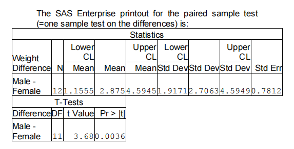
In this continuation of Example 1.2, where we compare the weights of male and female mice, we now consider that the pairs of mice are from the same litter. This changes the data into a set of differences. The test statistic for testing H0: μ1 = μ2 against Ha: μ1 ≠ μ2 is 3.68009, with a corresponding p-value of 0.00362526. This suggests that we reject the null hypothesis at significance levels above 0.4%, including the 1% and 5% levels.
This rejection occurs because the variation in weights within each litter is smaller than the overall variation in weights, indicating that mice from the same litter are more similar in weight compared to mice from different litters.
Summary of Hypothesis Testing
When conducting a statistical test, the initial step involves establishing a null hypothesis, indicating no difference, and an alternative hypothesis, which specifies the nature of the difference being investigated (either “not equal to” for a two-sided test, or “greater than” or “less than” for one-sided tests). These hypotheses are formulated in terms of population parameters, such as population means.
Next, you select an appropriate test statistic based on the nature of your data. This decision depends on whether you’re working with a single sample or multiple samples, as well as whether these samples are independent or dependent. While we’ve discussed the one-sample t-test, two-sample t-test, and paired sample t-test, there are numerous other tests available, some of which will be covered later.
Once you’ve chosen the test statistic, you compute its value using the sample estimates. Typically, statistical software calculates the exact probability of obtaining a test statistic of that magnitude if the null hypothesis is true. You then compare this probability to the significance level you’ve chosen, representing the risk of incorrectly rejecting the null hypothesis.
Alternatively, you can compare the test statistic to critical values from the appropriate distribution. For a given significance level, these critical values delineate the critical region where the null hypothesis is rejected if the test statistic falls outside.
In the case of a two-sided test, you can also derive conclusions from the confidence interval. However, it’s important to note that the confidence interval method is generally unsuitable for one-sided tests since it’s based on a two-sided argument.
References
Ott, R. L., Longnecker, M., & Schneider, G. (2019). Introduction to Statistical Methods and Data Analysis (7th ed.). Cengage Learning.
Field, A. (2013). Discovering Statistics Using IBM SPSS Statistics (4th ed.). Sage Publications.
Montgomery, D. C., Runger, G. C., & Hubele, N. F. (2018). Engineering Statistics (6th ed.). Wiley.
De Veaux, R. D., Velleman, P. F., & Bock, D. E. (2018). Intro Stats (5th ed.). Pearson.
Casella, G., & Berger, R. L. (2002). Statistical Inference (2nd ed.). Duxbury Press.