One common question statisticians face is, “How big of a sample do I need?” Answering this question isn’t straightforward and depends on various factors and assumptions.

The first thing a statistician will ask is, “What do you mean by ‘how large a sample’—large for what purpose?” For instance, detecting a very small difference, like 0.01, between two means requires a much larger sample size than detecting a larger difference, say 1.0. The goal, especially in testing for a difference between two means, is to use a sample size large enough to construct a confidence interval for the mean that allows for detecting the required difference. Essentially, the aim is to select a sample size (denoted as “n”) large enough so that the test statistic exceeds the critical value.

Let’s start by examining the simplest scenario to grasp the fundamental concepts before delving into more complex situations. This scenario involves the one-sample t-test, where the numerator of the test statistic is (x – μ).

Deciding on the sample size for any experiment involves a blend of statistical analysis and practical judgment. Often, the sample size is determined by factors like the number of available subjects, budget constraints, or time limitations. Even when practical constraints dictate the sample size, conducting sample size calculations can still be valuable. These calculations help assess whether the experiment or survey is worthwhile by indicating the size of differences one can likely detect with the proposed sample size. This information allows researchers to evaluate whether the expected outcomes meet the goals of the study.

In a well-designed study, it’s crucial to determine the sample size required to detect meaningful differences beforehand. For instance, a study examining 71 negative clinical trials in medical literature discovered that 50 of these trials would have overlooked a 50% improvement due to inadequate sample sizes. Another study analyzing 67 published clinical trials found that only 12% of them adequately addressed sample size considerations.

Opting for an excessively large sample size can lead to increased workload and potential wastage of resources. Conversely, choosing a sample size that’s too small might result in missing important differences or failing to detect any differences altogether. In cases where the sample size is too small, the experiment may yield no useful information, rendering the effort, resources, and participants or materials involved completely wasted.

For surveys, insufficient sample sizes can produce results indicating significant differences that are actually not statistically significant. In situations involving animals, both using too few or too many animals can be considered unethical.

Here are a couple of real-life examples where errors occurred due to inadequate consideration of sample size determination:

Thalidomide Tragedy: In the late 1950s and early 1960s, thalidomide was widely prescribed to pregnant women to alleviate morning sickness. However, it was later discovered that thalidomide caused severe birth defects in thousands of babies. The tragedy occurred because the initial safety testing of thalidomide did not involve a sufficiently large sample size to detect rare but serious side effects. As a result, the harmful effects of the drug were not adequately identified before it was widely distributed.

False Positive Results in Medical Screening Tests: In medical screening tests, such as mammograms or prostate-specific antigen (PSA) tests, inappropriate sample sizes can lead to false positive results. For instance, if a small sample size is used in a study evaluating the effectiveness of a new screening test for breast cancer, the test may appear to be highly accurate in detecting cancer. However, when the test is applied to a larger population, its accuracy may decrease, leading to unnecessary anxiety and medical procedures for patients who receive false positive results.

Public Opinion Polls: In political polling, sample size is crucial for accurately predicting election outcomes. If a pollster uses a small sample size, their results may not be representative of the entire population, leading to inaccurate predictions. For instance, in the 1936 U.S. presidential election, the Literary Digest conducted a poll with a large sample size but failed to account for selection bias, resulting in an incorrect prediction of the election outcome.

Product Testing: In 1985, Coca-Cola introduced “New Coke,” a reformulation of its classic Coca-Cola formula. The decision to reformulate the iconic soft drink was based on extensive taste tests involving a relatively small sample size of consumers. These taste tests overwhelmingly favored the new formula over the original one.

However, when New Coke was launched nationwide, it faced immediate backlash from consumers. Despite the positive feedback from the taste tests, consumers expressed strong dissatisfaction with the new flavor, leading to widespread protests and boycotts.

The failure of New Coke was attributed in part to the small sample size used in the taste tests, which did not accurately represent the preferences of Coca-Cola’s broader consumer base. While the taste tests indicated that the new formula was preferred by those sampled, it failed to account for the emotional attachment consumers had to the original Coca-Cola formula.

These examples illustrate how inadequate sample size determination can have practical consequences in various fields, ranging from political polling to product testing and manufacturing. By carefully considering sample size requirements, researchers and practitioners can minimize errors and produce more reliable results.

Sample size for a single sample

First, let’s talk about testing a single sample. We’re checking if the sample’s average (represented by μ) matches a specific value (μ₀) or not. We’re assuming we already know the population’s standard deviation (σ). If our sample size is big enough, we can use the normal distribution. So, our confidence interval for the average (μ) is calculated using the formula: x ± z₁₋ₐ/₂σ/√n. Here, z₁₋ₐ/₂ is a value from the normal distribution based on the level of significance (denoted by α). This interval stretches above and below our sample average (x) by a certain distance (D), where D = z₁₋ₐ/₂σ/√n. This means that if we’re testing at a certain level of significance (α), we won’t be able to detect any difference smaller than D away from our sample average (x).

Now, let’s consider a scenario where we take a sample from a population with an average of μ₁ and test if it’s equal to μ₀. We can only reject the null hypothesis if the difference between μ₀ and μ₁ is bigger than half of the width of the confidence interval, which is D. So, D represents the smallest difference we can detect at a certain level of significance (α), given σ and the sample size (n).

As we increase the sample size (n), the confidence interval becomes narrower because the square root of n in the denominator increases, meaning we’re dividing by a larger number. Consequently, with larger sample sizes, we can detect smaller differences. This highlights the importance of specifying the size of the difference we aim to detect when determining the required sample size.

When we talk about determining if two groups are different, we’re not aiming to prove that their estimated means are exactly the same (which is practically impossible due to minute variations). Instead, we’re using the samples to understand what’s happening in the underlying populations. Our focus is on detecting a “real” difference that holds practical significance. Typically, we have a range of differences in mind that would be meaningful or beneficial.

Consider the case of testing a new fertilizer’s impact on tomato plant yield compared to a standard fertilizer. We’re interested in whether it leads to a higher yield, specifically by at least 2 kilograms per plant per season, as anything less wouldn’t justify the cost. However, we’re not concerned with detecting an unrealistically large increase, such as 50 kilograms.

Our goal is to determine a sample size large enough to detect a 2-kilogram increase. If this requires, for instance, 50 plants, the experiment is feasible. But if it demands an impractical sample size, like 5 million plants, the experiment may not be feasible. We also need to consider practical limitations, like available land and plant spacing.

The formula linking sample size to the size of the effect (in a single-sample scenario) is:

Let’s break down each element of the formula:

1. Sample size (n): This is usually what we’re trying to figure out. Sometimes, practical limitations determine the sample size, and we’re interested in knowing the smallest effect (D) we can detect with the given sample size.

2. Size of effect (D): This is the smallest effect that’s worth detecting, meaning any larger effect is also valuable. It heavily influences the sample size needed. It’s essential to note that statistical significance doesn’t always align with practical importance. Statistical significance focuses on the likelihood that random chance alone could produce a difference of this size, while practical importance concerns the usefulness of that difference. With a large enough sample, we can detect very small differences, but these might not be practically meaningful. For example, detecting a slight increase in exam scores might not be worth the effort of extra lessons.

3. Significance level (α): This indicates the risk you’re willing to take of incorrectly concluding there’s a difference when there isn’t one (type I error).

4. Standard deviation (σ) of the population: This is the standard deviation of the population assumed under the null hypothesis, often representing the standard treatment. It can be estimated from previous data, scientific literature, or personal knowledge. Estimating this parameter can be challenging, especially without prior studies in the area. One might want to use the estimated standard deviation from the sample, but it’s a catch-22 situation since the sample can’t be drawn until the sample size is specified. Exploring the effect of varying the assumed standard deviation can be helpful, looking at its implications on sample size (n) or the size of effect (D).

One solution to this issue is to estimate the standard deviation from a pilot survey. However, conducting a pilot survey requires permission and funding, and sample size calculations are necessary for it as well. Additionally, small surveys may not provide accurate estimates of the standard deviation, and these estimates might be less useful than educated guesses. Therefore, this approach is often impractical.

Another approach is to specify the ratio D/σ instead of both D and σ, indicating that we aim to detect an effect of D/σ standard deviations. However, this approach may not always be helpful in many situations.

There’s one scenario where knowledge of the standard deviation isn’t needed, and that’s when dealing with proportions, but this will be dealt with in the course on Proportions.

It might be surprising, but the size of the population (N) doesn’t factor into sample size calculations. This is because populations are usually large compared to sample sizes. In such cases, the ratio of the sample size to the population size (n/N) is so small that even doubling the sample size doesn’t make a significant difference. Population size only becomes important if it’s small relative to the sample size, like when you need to sample a significant portion (e.g., 10% or 20%) of the population.

Situations where population size matters more include auditing, sampling rare species, or estimating the proportion of time a rare event occurs. For instance, when testing for botulism in a batch of tins where it’s rare (maybe 1 in 1000), you might need to sample a large portion of the batch (like 80%) to be certain of detecting a contaminated tin, which may not be feasible.

For auditing or when dealing with rare populations, more advanced statistical methods are needed. These scenarios aren’t covered in this text, but resources like Cochrane and Fleiss et al. provide further insights.

Example 3.1 (Continuing from example 2.2)

In the previous example about piglets fed a specific diet, let’s say we want to detect a difference of 50 grams in weight gain compared to a standard diet with a gain of 200 grams. This means we want the confidence interval to be narrow enough to detect a 50 gram difference in either direction. In other words, we want the difference (D) to have a maximum of 50 grams.

To find the number of piglets (n) needed for the experiment, we set up an equation: 50 = z₁₋ₐ/₂σ/√n. We still need to choose values for σ and α. In our previous assumption, we knew the population standard deviation (σ) was 120 grams, so we’ll use that. If we want to test at the 5% level (implying α/2 = 0.025), this corresponds to z₁₋ₐ/₂ = 1.96.So, we want to find the sample size (n) such that: ​

Thus, we need a sample size of 23 to detect a 50-gram difference at the 5% significance level, assuming a population standard deviation of 120 grams. The rounding up ensures that we have at least 22.13 units, and since we can’t have a fraction of a unit, we round up to 23.

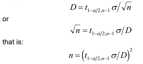
When the experiment is conducted, the assumed population standard deviation is rarely used. Instead, the sample standard deviation is utilized along with the t-test:

The nul

l hypothesis is rejected if the test statistic exceeds (in absolute value) the critical value t1−α/2,n−1​. Therefore, the z1−α/2​ in the previous calculations should be substituted with t1−α/2,n−1​, leading to the equation:

This introduces a complication because the critical value for the t distribution varies with sample size. Therefore, we need to obtain the solution through iteration, trying several values, rather than a straightforward calculation as before. Here’s how we proceed:

• Let n1​ be the sample size obtained using the critical value from the normal distribution, and n2​ be the correct estimate.
• We know that the critical value from a t-distribution is larger than that from the normal distribution, eventually becoming equal for large sample sizes.
• Therefore, the sample size obtained using the t-distribution will be larger than or equal to that obtained from the normal distribution.
• Thus, the estimate of the sample size obtained using the normal distribution will be smaller than the final sample size estimate.
• Using the sample size n1​, determined from the calculation using the normal distribution critical value, we look up the corresponding critical value for the t distribution. This results in a t critical value larger than the one for the correct sample size: 1−α/2,n1​−1​>t1−α/2,n2​−1​.
• Therefore, using n1​ will give us a sample size estimate n∗ that is too large, and the true sample size will lie between n1​ and n∗.
• We start with n1​, find n∗∗, and then try numbers in between to find n∗. The final estimate is reached when both sides of the equation are satisfied.